OCT 27, 2025
Toward Predictable Borrowing in DeFi with the Arkis Dynamic Spread Model
Traditional utilization-based models make borrowing costs noisy and unpredictable, undermining institutional strategies. Arkis solves this with our Dynamic Spread Model, anchoring rates to collateral yields and target spreads for predictable lending markets.
Author: Oleksandr Proskurin, CPO and Сo-founder at Arkis


1
Introduction
The State of Borrowing in DeFi
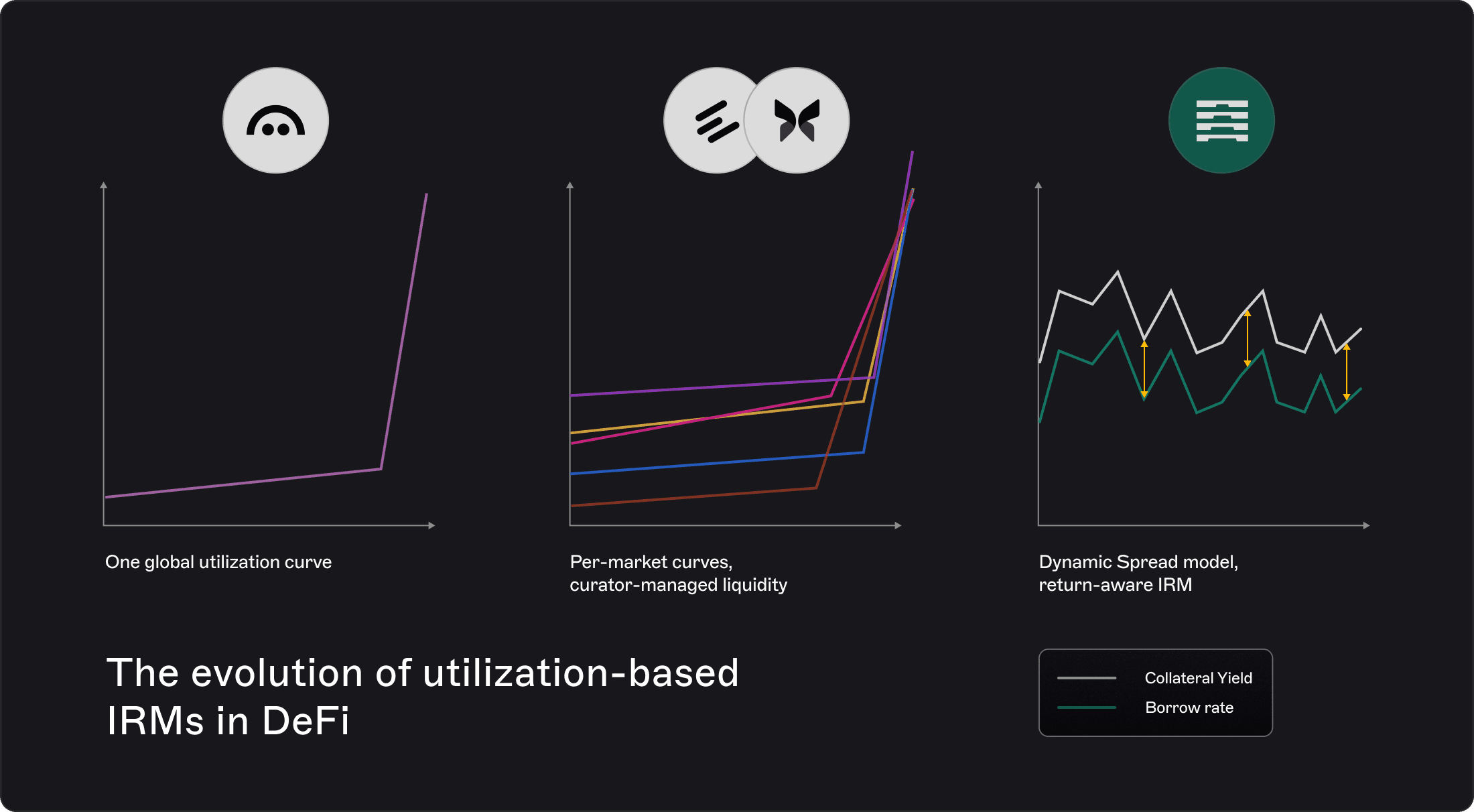
Interest rate models (IRMs) are the foundation of on-chain credit markets. They determine how much a borrower pays and how much a lender earns, shaping the dynamics of everything from retail yield farming to complex institutional arbitrage. Over the past years, utilization-based IRMs have emerged as the default design across major lending protocols such as Aave, Euler, and Morpho.
At their core, these models are driven by utilization — the ratio of borrowed assets to total supplied liquidity. When utilization is low, borrow rates remain low, encouraging new borrowing. As utilization rises, borrow rates increase sharply, incentivizing repayment and new supply until equilibrium is restored.
Borrow rates stay low at low utilization, then rise sharply as utilization increase — driving repayment, new supply, and restoring equilibrium.
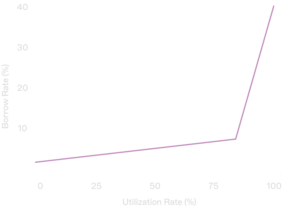
This mechanism is intuitive, simple to implement, and has proven effective at keeping lending pools solvent under volatile conditions. It also aligns with traditional supply-and-demand logic: scarce liquidity should cost more.
Because of these properties, utilization-based models have become the backbone of DeFi borrowing. Yield farmers, loopers on Aave, and even institutional hedge funds structure trades and capital strategies around the expectation that borrow costs will follow these utilization curves.
While utilization curves remain effective at maintaining solvency, they introduce noise and unpredictability that complicates risk management for professional borrowers.

The first successful example was Aave’s pure utilization curve, applied for each borrowed assets on the platform. Later iterations — Morpho and Euler — extended this idea by introducing market-specific utilization curves, where each pool’s cost of borrowing depends not only on utilization but also on how effectively curators manage supply liquidity in response to borrowing demand.
Yet as DeFi matures and institutional borrowers deploy looping and arbitrage strategies at scale, cracks in this paradigm are becoming more visible. While utilization curves remain effective at maintaining solvency, they introduce noise and unpredictability that complicates risk management for professional borrowers. For those who depend on stable financing costs, this instability can erode the viability of trades that would otherwise appear profitable.
In the following sections, we will explore these frictions in detail, and then introduce a new model — Arkis Dynamic Spread IRM — designed to deliver a more predictable and return-aware borrowing environment.

2
Challenges
Where Utilization-based Models Fail Borrowers
While utilization-based IRMs have provided the backbone for DeFi lending, they also introduce structural challenges that become particularly visible in fragmented liquidity environments like Morpho and Euler, where each market operates with its own utilization curve. For institutional borrowers and loopers, these challenges translate directly into noise, unpredictability, and operational inefficiency.
1
Noise in Borrow Rates
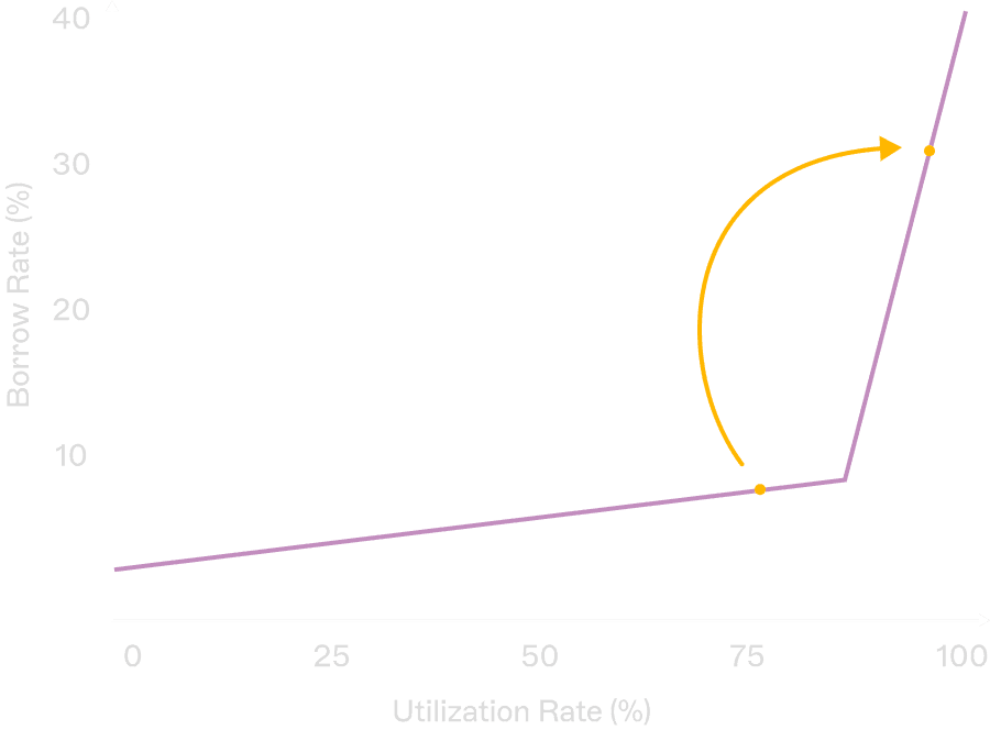
Borrow rates in utilization-based models are highly sensitive to small changes in utilization. The presence of a “kink” point — where rates accelerate sharply once utilization crosses a threshold — forces borrowers to self-assess their capacity before entering a position.
A trader may see significant free liquidity in the pool, but borrowing it in full can spike the utilization into the kink region.
The result: a sudden, disproportionate increase in borrow costs that can turn an otherwise profitable trade unviable.
This makes borrow costs less predictable and introduces noise into the return profile of leveraged strategies.
A trader may see free liquidity, but borrowing it all can push utilization into the kink—spiking costs and killing profits.
2
Liquidity Estimation Challenges
In theory, the amount of free liquidity in a market should reflect the potential capacity for new trades. In practice, it does not.
Borrowers cannot simply “fill” the available liquidity without materially altering the borrowing environment.
The kink mechanism means that liquidity is not linear: consuming the last portion of available supply radically changes rates.
As a result, “free liquidity” ≠ “usable liquidity.”
For asset managers, this forces constant recalibration of positions and often reduces effective trade capacity far below the headline liquidity number.
With the kink mechanism borrowers can’t just “fill” the pool without changing the environment. As a result, “free liquidity” ≠ “usable liquidity.”


3
Trade Crowding & Negative-sum Outcomes
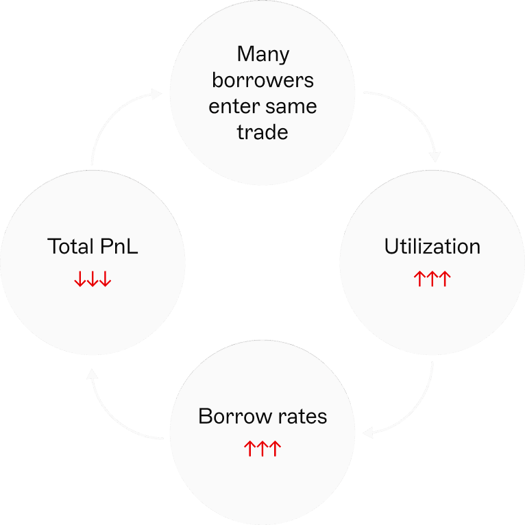
When multiple loopers or asset managers identify the same opportunity, they often rush into the same market.
This crowding effect drives utilization up.
Borrow rates spike simultaneously for all participants.
What looked like a high-yield trade turns into a lose-lose outcome: even early entrants may see their expected PnL evaporate as rates climb.
Instead of a stable environment for professional capital, this creates a game where traders must constantly monitor utilization and cycle in and out of leveraged loops depending on short-term borrow costs.
4
Over-reliance on Curators
In protocols like Euler and Morpho, curators are responsible for balancing liquidity across markets. While curators can theoretically stabilize utilization by adjusting incentives, in practice this creates additional uncertainty for borrowers:
Their ability to execute and sustain a strategy depends on how efficient the curator is at managing liquidity.
Borrowers cannot predict in advance how responsive curators will be to utilization spikes.
This introduces yet another hidden variable into the borrowing decision.
For institutional asset managers who require predictable cost of capital, this reliance on curator behavior creates friction and risk.
5
High-leverage Risk Amplification
For strategies involving leverage, utilization spikes are especially dangerous.
A trade that appears highly profitable at 60% utilization can flip to deeply unprofitable at 70% utilization.
Because utilization can shift quickly due to a single large borrower or multiple entrants crowding the same loop, leveraged borrowers bear asymmetric downside risk.
This forces managers to build costly buffers into their strategies or retreat to fixed-term loans where rates are more predictable.

Takeaway
Net Effect: Utilization as a Noisy Variable
Taken together, these challenges mean that utilization is not a clean or transparent input for professional borrowers. Instead, it becomes a hidden, noisy variable that must be estimated, predicted, and dynamically controlled. The burden shifts to asset managers, who must manage not only market risk but also liquidity-modeling risk — a burden that utilization-based IRMs were never designed to impose.

3
Our Approach
Introducing the Arkis Dynamic Spread Model
Utilization-based approach was a natural choice where the protocol had to create a mechanism which does not lock in lenders in lending pools. With 100% utilisation all the capital is borrowed and the lenders were locked in which creates serious structural risk for liquidity providers. The key assumption here is that the borrower can be any actor in DeFi - as a result malicious borrowers could take all liquidity from the pool and lock in lenders. As a result, utilisation kink was a natural mechanism to penalise borrowers from borrowing too much to provide lenders with liquid and safe yield vehicle.
However, at Arkis all borrowers are regulated and KYCed asset managers - as a result there is no need in protecting lenders from being locked by malicious actors. Furthermore, most of the lenders (due to the non-active nature of lending) would prefer to lock in their capital for higher yield. As a result, in institutional lending where borrowers intents are clearly understandable there is no need to create “protection” mechanism in a form of utilization curve.


Arkis goes beyond utilization by adding three parameters that make borrowing costs predictable, tied to returns, and suited for institutions.
For loopers and arbitrageurs, the central calculation is simple: the spread between collateral yield and borrow rate. The higher the spread, the more attractive the opportunity. In practice, however, utilization-based IRMs make this spread noisy and unpredictable, forcing traders to guess whether a loop can be sustained once borrowing begins.
The Arkis Dynamic Spread model takes a different approach. Instead of relying solely on utilization — a blunt proxy for supply and demand — Arkis introduces three new parameters that make borrowing costs more predictable, return-aware, and aligned with institutional needs.
1
Collateral Expected Yield
The first and most important input is the expected return of the collateral asset. Since collateral is typically used in loop strategies, this expected yield determines the potential profitability of the trade.
For example:
With Pendle PTs, the implied APY is already known in advance, making expected yield straightforward to measure. For carry trades, expected yield can be estimated as:
Expected Yield = 0.5 * (Spot yield + Funding Yield from Futures)
A borrower’s P&L is typically expressed as:
P&L = Collateral Yield + (Collateral Yield − Borrow Rate) × Leverage
By grounding the model in expected yield rather than raw utilization, Arkis directly ties borrowing costs to the economics of looping.
2
Target Spread
The second parameter is the target spread — the minimum delta between collateral yield and borrow rate that makes a trade worthwhile for the borrower.
This is modeled as an exponential function:
Where:
Collateral Yield is Collateral Expected Yield
Min_Spread is a minimum expectable spread by the borrower to be involved in looping activities.
Max_Spread is a maximum possible spread which would make sense for the borrower to loop the trade as much as possible.
Senstitivity defines how responsive spread value is relative to change in Collateral Yield.
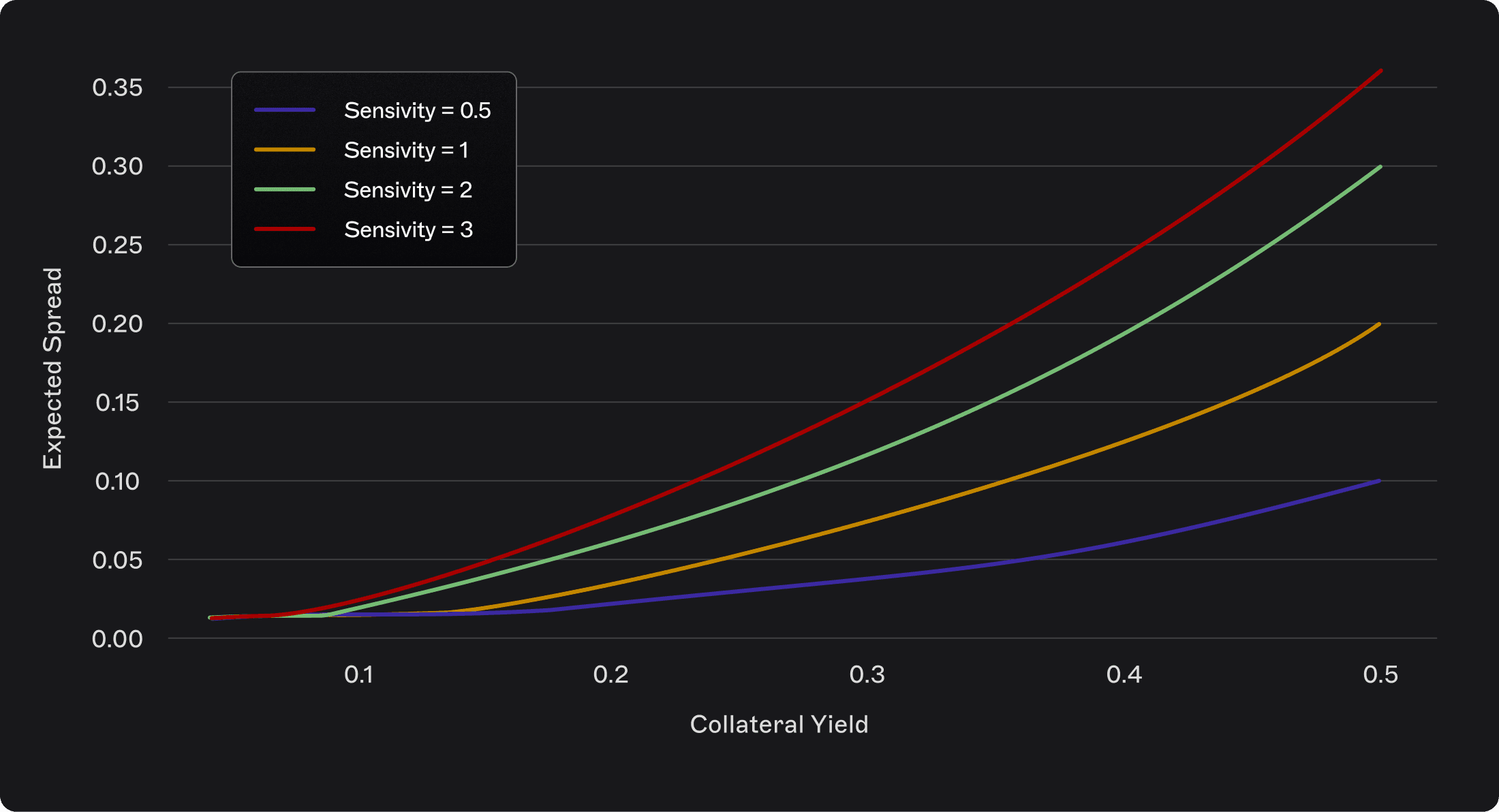
Expected target spread as a function of different sensitivity parameter values
If collateral yield is high (e.g., 15%), borrowers demand a higher spread (e.g., at least 3%).
If collateral yield is modest (e.g., <10%), borrowers are willing to accept a smaller spread (e.g., 2%).
Whatever low the yield is, borrowers are expecting min_spread to be interested to take the looping risk.
In other words, higher yields justify higher spread requirements.
3
Minimum Lending Rate
The third parameter accounts for the minimum return lenders require to justify lending against a specific collateral. Even with a “safe” asset such as USDe, where PT yields may be 7%, lenders will not deploy capital unless they receive a baseline return (typically ~5%) that compensates for protocol and counterparty risk.
This parameter functions as a risk-free rate floor, ensuring lenders are not forced to accept below-market returns.
4
Performance Fee Sharing Logic
Arkis Protocol applies 10% performance fee. However, instead of naively charge lender or a borrower, Arkis IRM introduces a fair fee-splitting mechanism based on utilization:
At 50% utilization, the performance fee is split evenly between lenders and borrowers.
At high utilization, borrowers bear more of the fee.
At low utilization, lenders bear more of the fee.
This ensures that the system responds fairly to market conditions, without destabilizing the underlying economics of looping.
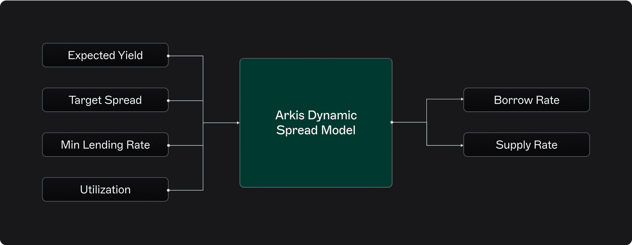
Inputs → Arkis IRM → Outputs
Arkis Dynamic Spread Formulas
Taking all together, over time, lend/borrow rates are dynamically updated with utilization feedback:
Definitions
protocol performance fee (10-20%)
minimum lending rate
expected collateral yield at time t
utilization ratio at time t
exponential sensitivity parameter defining target spread
minimum (base) spread for the borrower to be interested in looping
upper cap on spread to prevent excessive borrower cost
target spread at time t
Target spread determination

Reference Rate Calculation

Performance Fee and Effective Rates

Why This Matters
The result is a model where:
Borrowers can be confident that borrow costs will never exceed collateral expected yield.
Lenders receive a minimum guaranteed return plus utilization-adjusted fees.
Lenders are fairly exposed to collateral expected yield. Higher yields for borrowers means higher lending rates for borrowers while the effective spread for looping is also higher.
The system combines the predictability of fixed-term models with the responsiveness of dynamic rates.
For loopers and institutional borrowers, this creates a stable and transparent environment — eliminating the hidden noise and guesswork introduced by utilization-only IRMs.

How it works
Mechanics of the Arkis Model
This design integrates utilization in a subtler way than traditional IRMs:
If utilization is low, it signals weak borrower interest → reference rate decreases, creating more favorable arbitrage conditions.
If utilization is high, it signals strong borrower demand → borrow rate rises slightly, with a larger share of fees passed on borrowers.
In simple terms, utilization is no longer the main driver of costs but a feedback signal that adjusts spreads based on real borrower demand.


4
Arkis in Action
Quantitative Comparison vs. Utilization Models
To demonstrate how Arkis performs in practice, we analyze a concrete case study: a Pendle PT USDe Sep 2025 looping trade. For loopers, the key metric is straightforward:
Net Spread = Collateral Yield − Borrow Rate
As long as the spread remains positive, looping makes sense; once it turns negative, borrowers are forced to unwind positions.
We compare four protocols: Aave, Euler, Morpho, and Arkis — examining their lending (supply) and borrowing (looping) dynamics across the same trade.
1
Historical Collateral Yield (Pendle PT Implied APY)
We begin with the baseline: the Pendle PT USDe implied APY over time. This rate represents the return a borrower can earn by supplying their collateral into the Pendle market. Periods of drawdown — such as the sustained dip in early August, shown in the chart — compress the profitability of looping trades, while the mid-August upswing expands margins and creates more favorable conditions.
These dynamics establish the “earning side” of the loop: when yields climb, loopers have more room to generate positive spread; when yields soften, the trade relies heavily on borrowing costs remaining contained.

Pendle USDe Sep 2025 Implied APY plot
2
Historical Borrow & Lend Rates Across Protocols
Next, we overlay the borrowing and lending rates from the four protocols.
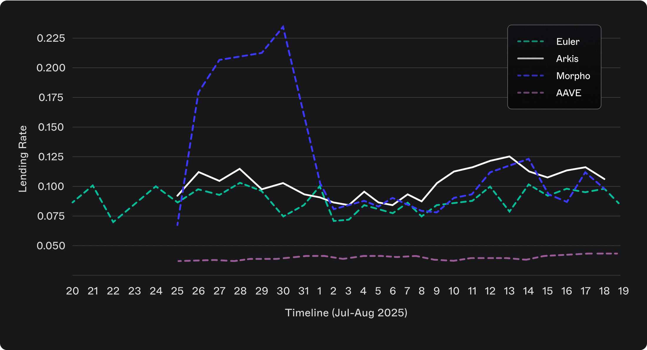
Lending Rates Comparison
Arkis, Euler, and Morpho all display lending rates that move in a similar range, reflecting a model where lenders are rewarded for the specific risks they choose to take. This structure ensures that those who provide liquidity against collateral like Pendle USDe are compensated fairly.
Aave, by contrast, applies a single-rate model across all assets. While this creates deep liquidity and attractive conditions for borrowers, it leaves lenders under-incentivized, since they are not paid more for accepting higher-risk collateral.
Borrowing rates mirror these dynamics. Arkis, Euler, and Morpho borrowers face costs aligned with lender expectations, whereas Aave borrowers consistently benefit from artificially low rates. The notable outlier is Morpho’s late-July spike in borrowing costs, which would have disrupted ongoing looping strategies by suddenly erasing profitability.
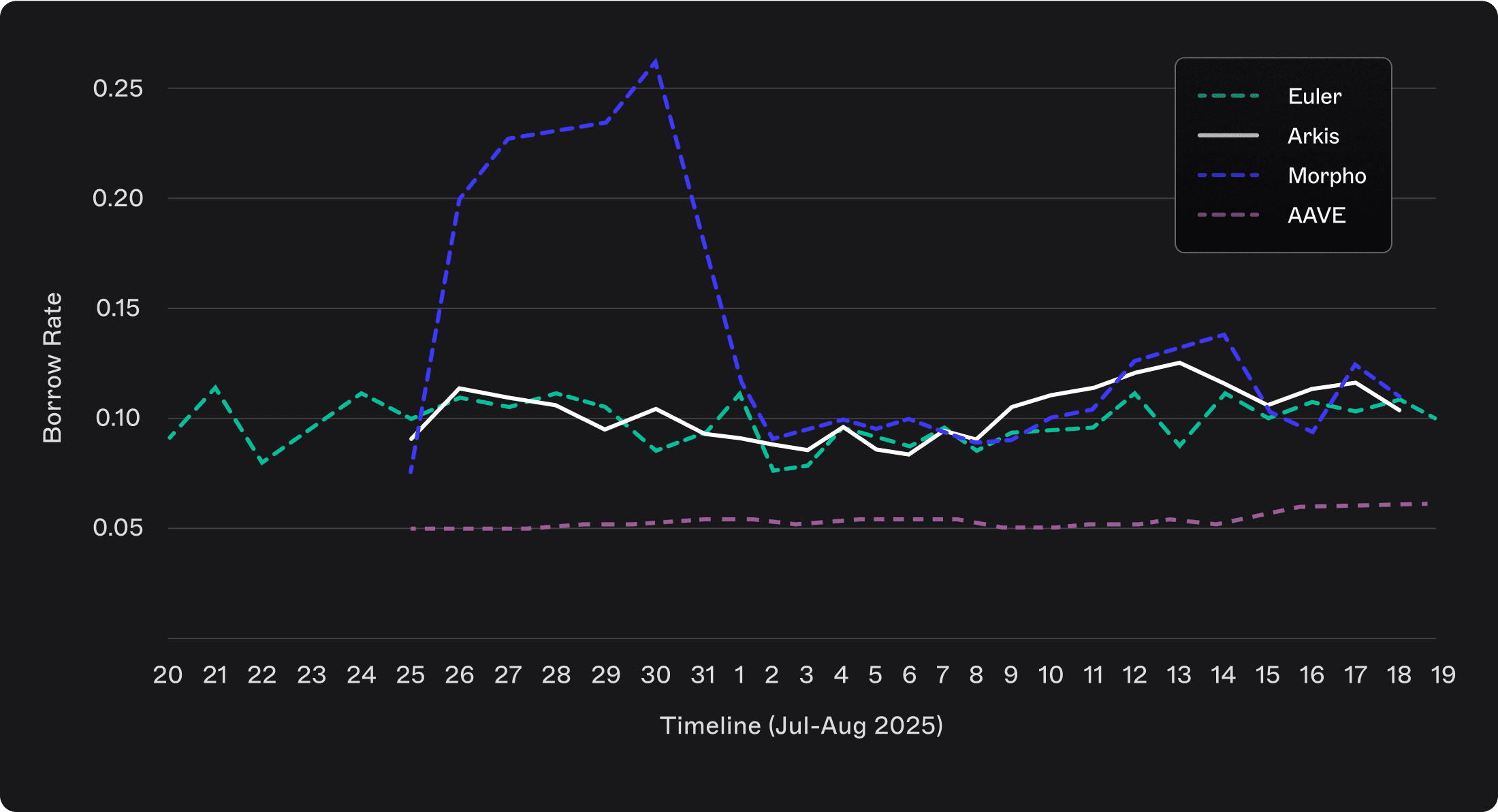
Borrow Rates Comparison
We can see that borrow rates dynamics looks pretty similar with the lending rates, however Morpho’s borrow rate show a spike from the end of July which would cause issues for asset managers.
3
Net Spread Analysis (Collateral Yield – Borrow Rate)
In this section, we examine the net spread — the difference between what borrowers pay and what lenders earn — across major protocols. This metric captures the true profitability of looping and borrowing strategies. A stable and positive net spread indicates sustainable conditions, while a volatile or negative spread signals potential liquidation risks.
The chart below tracks how the net spread evolved over time for each protocol, revealing differences in market structure and risk management.

Net Spread = Pendle APY - Borrow Rate
The decisive factor for loopers is the net spread—the margin between what their collateral earns and what they pay to borrow. A positive spread supports sustainable looping, while a negative one forces liquidations or early unwinds. Looking across protocols, each model produces distinct outcomes for asset managers:
Arkis IRM: Spread remains consistently positive and stable. Euler: Higher spreads on average, but volatile;
AAVE: Highest spread for borrowers, deep market liquidity but lenders are actually the one who “pay” for such a good arbitrage opportunity for the borrowers.
Morpho: Spread crosses into negative territory, forcing asset managers to unwind profitable trades prematurely.
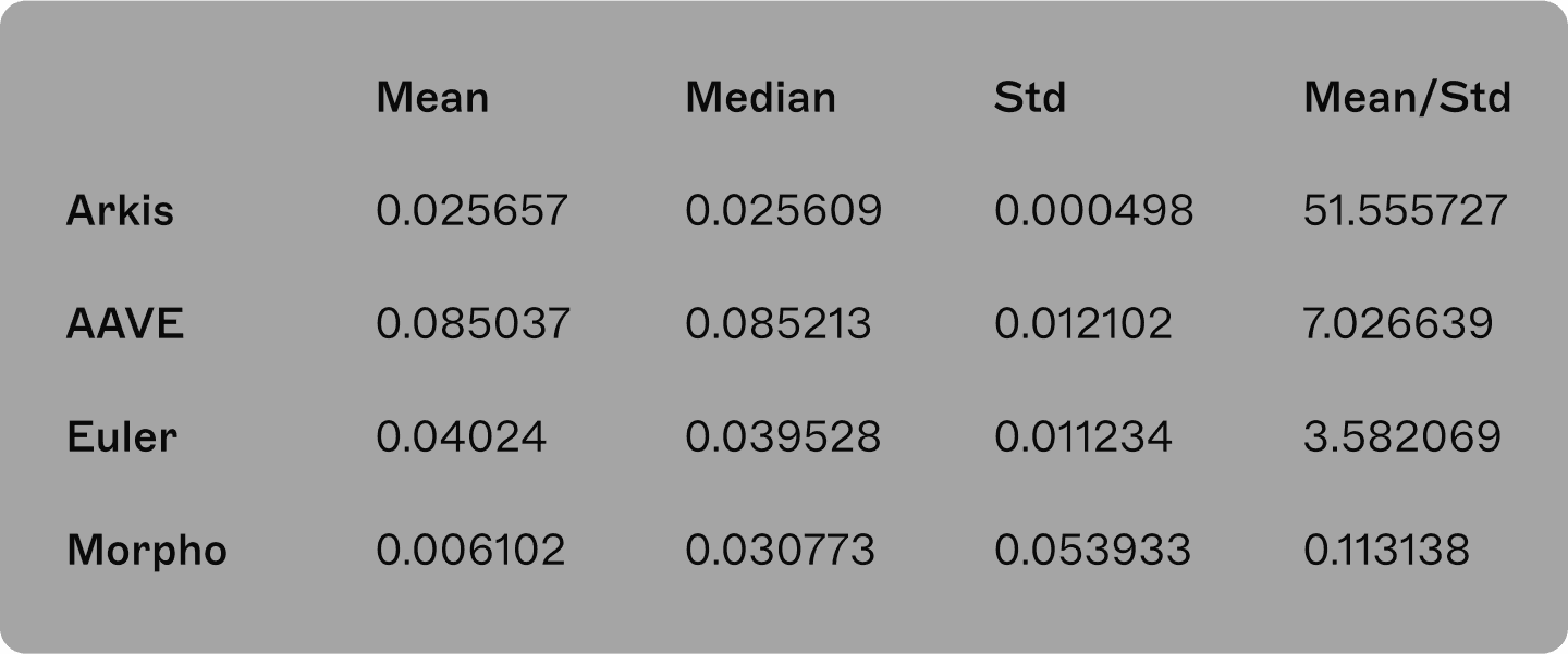
To quantify the performance differences, we analyzed the mean, median, and standard deviation of the net spread across protocols. These metrics provide a clear picture of both profitability and stability, the two defining aspects of net spread, which is the most important determinant of sustainable looping.
Even though Arkis provided the lowest average and median spread compared to AAVE, Euler and Morpho, it provided a much more stable arbitrage environment (Arkis has substantially lower standard deviation of spread and by far the biggest value of “stability score” - mean/standard deviation” of net spread).
By taking a look at Net Spread as a function of potential utilization we can also see positive signs:
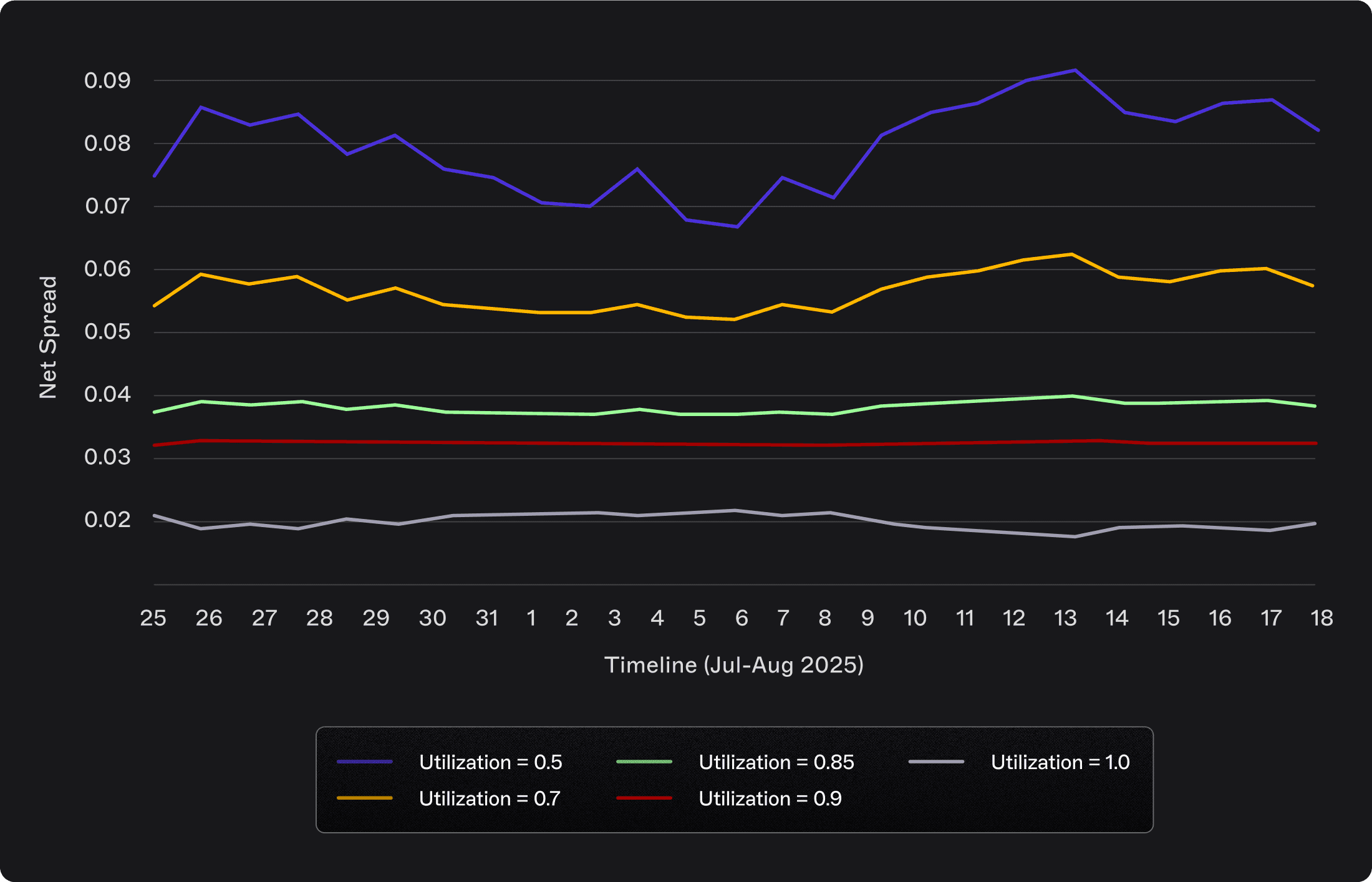
Net Spread dynamics as a function of utilization
We can also see that even at 100% utilization - borrower’s net spread of arbitrage does not fall below 0 which creates a safe environment for taking leveraged positions.
Lending rates analytics:
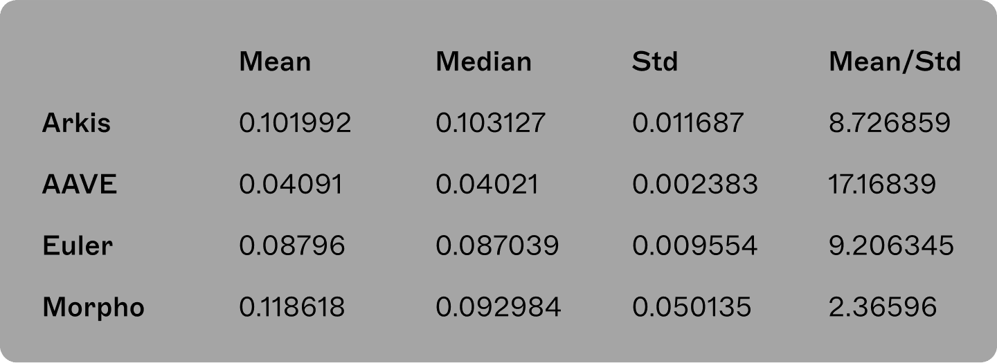
At the same time, for lenders Arkis provided the biggest median supply APY with the second largest average. It means that borrowers have a stable environment for margin trading while lenders are compensated fairly.
For institutional borrowers, the conclusion is clear:
Stability and predictability -> chasing the occasional higher spread.
Arkis IRM ensures scalability of capital without destabilizing costs.
For institutional lenders:
Being fairly rewarded for financing margin trading for the specific collateral type.
Being exposed to increasing yield of collateral which creates more deposit incentives.
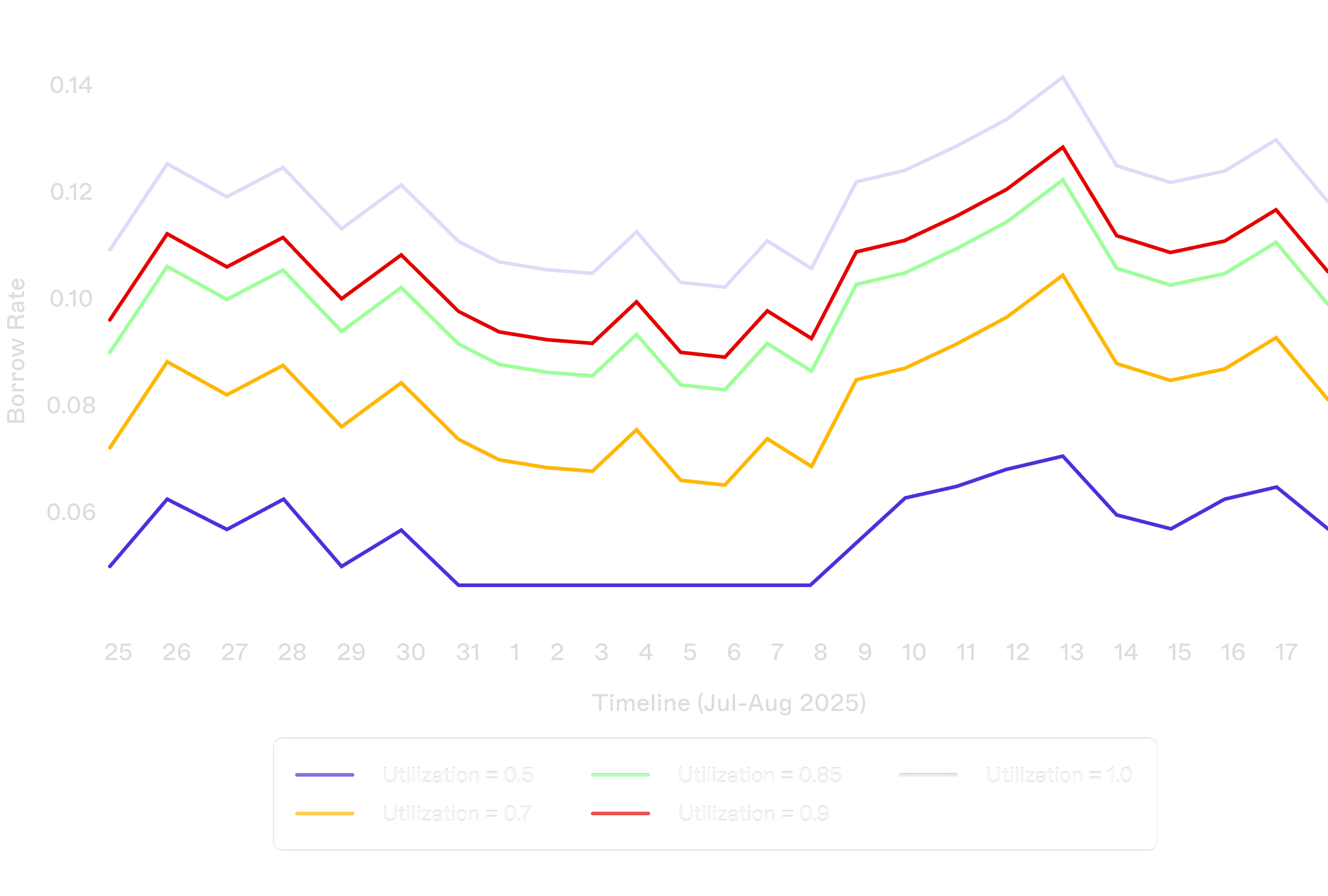
Borrow Rate Sensitivity to Utilization
Finally, we examine how borrow rates evolve as a function of utilization.
Traditional models: Sharp kinks — small jumps in utilization lead to large jumps in cost.
Arkis IRM: Borrow rates remain smooth, shallow, and anchored to expected returns — even at high utilization levels.
This fulfills the design objective: Make borrow rates less sensitive to utilization. Make them more sensitive to expected trade returns.

Takeaway
Case Study Key Insights
For Borrowers:
Arkis IRM creates an environment where “it always makes sense to borrow.”
Even if the spread is slightly smaller than Euler or Aave at times, it is stable, scalable, and predictable — qualities essential for institutional adoption.
For Lenders:
Lending returns remain tied to market conditions: higher when collateral yields increase, lower when they fall.
The minimum reference rate ensures lenders are never forced into uneconomic outcomes.
For Market Structure:
By anchoring to expected yields rather than pure utilization, Arkis IRM behaves more like mezzanine debt — a layer where borrower returns directly influence lending rates.
This bridges the best of two worlds: fixed-term predictability with dynamic, utilization-aware adjustments.

5
Conclusion
Toward Predictable Borrowing in DeFi
Utilization-based interest rate models have powered DeFi lending since the earliest days of Aave. They are simple, intuitive, and effective at ensuring solvency. But as DeFi has matured — and as institutional borrowers deploy looping and arbitrage strategies at scale — the limitations of these models have become increasingly visible.
From noisy borrow rates, to hidden liquidity constraints, to over-reliance on curators, utilization curves introduce uncertainty that undermines the stability professional asset managers need. For leveraged strategies, this unpredictability can flip profitable trades into losses, forcing borrowers into constant monitoring and premature unwinds.
The Arkis Dynamic Spread model addresses these frictions by anchoring borrowing costs to the economics of the trade itself:
Collateral Expected Yield sets the foundation.
Target Spread ensures trades remain worthwhile.
Minimum Lending Rate protects lenders with a guaranteed baseline return.
Utilization is retained, but as a feedback mechanism — smoothing rates rather than dictating them.

DeFi’s new approach
Results of the Arkis Model
Borrowers gain predictable, stable borrowing costs tied to real yield opportunities.
Lenders earn returns that flex with market conditions, without ever falling below risk-adjusted minimums.
Markets achieve greater scalability and efficiency, enabling deep liquidity pools suitable for institutional capital.
In practice, this means that with Arkis IRM, it always makes sense to borrow. The spread remains stable, trades remain scalable, and both sides of the market are aligned.
As DeFi continues to evolve, models like Arkis Dynamic Spread lay the groundwork for a new era of on-chain credit — one where predictability, efficiency, and institutional confidence are built into the core design of lending markets.